Solving a simple PDE
The following problem also exists as an notebook. Here we give a beginner-friendly introduction to TorchPhysics, going over all the basic concepts and steps.
We introduce the library with the aim to solve the following PDE:
For comparison, the analytic solution is \(u(x_1, x_2) = \sin(\frac{\pi}{2} x_1)\cos(2\pi x_2)\).
Generally, the first step is to define all appearing variables and giving them a name.
In TorchPhysics all input variables are considered as variables that have to be named,
but also the solution functions.
From a mathematical point of view we essentially define to what space these variables
belong (for example \(x \in \mathbb{R}^2\)). From a more applied point, we just set the name
and dimension of our input and output values:
import torchphysics as tp
X = tp.spaces.R2('x') # input is 2D
U = tp.spaces.R1('u') # output is 1D
Next up is the domain, in our case a simple square. There are a lot of different domains
provided in TorchPhysics (even logical operations and time dependencies are possible),
these will be introduced further later in the tutorial and can be found under the section
domains.
Usually a domain gets as an input the space it belongs to (here our ‘x’) and some different parameters that depend on the constructed object. For a parallelogram, for example the origin and two corners.
square = tp.domains.Parallelogram(X, [0, 0], [1, 0], [0, 1])
Now we define our neural network, that we want to train. There are different architectures pre implemented, but since we build upon PyTorch one can easily define custom networks and use them.
For this example we use a simple fully connected network.
In TorchPhysics all classes that handle the networks are collected under the models section.
model = tp.models.FCN(input_space=X, output_space=U, hidden=(50,50,50,50,50))
The next step is the definition of the training conditions. Here we transform our PDE into some residuals that we minimize in the training. From an implementation point, we stay close to the original (mathematical) PDE and to the standard PINN approach.
Here we have two different conditions that the network should fulfill, the differential equation itself and the boundary condition. Here, we start with the boundary condition:
For this, one has to first define a Python-function, that describes our trainings condition. As an input, one can pick all variables and networks that appear in the problem and were defined previously, via the
spaces. The output should describe how well the considered condition is fulfilled. In our example, we just compute the expected boundary values and return the difference to the current network output. Here,uwill already be the network evaluated at the pointsx(a batch of coordinates). Internally, this will then be transformed automatically to an MSE-loss (which can also be customized, if needed).We also need to tell on which points this condition should be fulfilled. For this TorchPhysics provides the
samplerssection. Where different sampling strategies are implemented. For the boundary condition we only need points at the boundary, in TorchPhysics all # domains have the property.boundarythat returns the boundary as a new domain-object.
import torch
import numpy as np
# Frist the function that defines the residual:
def bound_residual(u, x):
    bound_values = torch.sin(np.pi/2*x[:, :1]) * torch.cos(2*np.pi*x[:, 1:])
    return u - bound_values

# the point sampler, for the trainig points:
# here we use grid points any other sampler could also be used
bound_sampler = tp.samplers.GridSampler(square.boundary, n_points=5000)
bound_sampler = bound_sampler.make_static() # grid always the same, therfore static for one single computation
Once all this is defined, we have to combine the residual and sampler in a condition.
These condition handle internally the training process.
Under the hood, they have the following simplified behavior (while training):
Sample points with the given sampler
Evaluate model at these points
Plug points and model output into the given residual
Compute corresponding loss term
Pass loss to the optimizer
In TorchPhysics many different condition types are pre implemented
(for including data, integral conditions, etc.).
Here we use the PINN approach, which corresponds to a PINNCondition:
The same holds for the differential equation term. Here also different operators are implemented,
that help to compute the derivatives of the neural network.
They can be found under the utils section.
# Again a function that defines the residual:
def pde_residual(u, x):
    return tp.utils.laplacian(u, x) + 4.25*np.pi**2*u

# the point sampler, for the trainig points:
pde_sampler = tp.samplers.GridSampler(square, n_points=15000) # again point grid
pde_sampler = pde_sampler.make_static()
# wrap everything together in the condition
pde_cond = tp.conditions.PINNCondition(module=model, sampler=pde_sampler,
                                       residual_fn=pde_residual)
The transformation of our PDE into a TorchPhysics problem is finished. So we can start the training.
The last step, before the training, is the creation of a Solver. This is an object that inherits from the Pytorch Lightning LightningModule. It handles the training and validation loops and takes care of the data loading for GPUs or CPUs. It gets the following inputs:
train_conditions: A list of all train conditions
val_conditions: A list of all validation conditions (optional)
optimizer_setting: With this, one can specify what optimizers, learning, and learning-schedulers should be used. For this, there exists the class OptimizerSetting that handles all these parameters.
# here we start with Adam:
optim = tp.OptimizerSetting(optimizer_class=torch.optim.Adam, lr=0.001)

solver = tp.solver.Solver(train_conditions=[bound_cond, pde_cond], optimizer_setting=optim)
Now we define the trainer, for this we use Pytorch Lightning. Almost all functionalities of Pytorch Lightning can be applied in the trainings process.
import pytorch_lightning as pl

trainer = pl.Trainer(gpus=1, # or None if CPU is used
                     max_steps=4000, # number of training steps
                     logger=False,
                     benchmark=True,
                     checkpoint_callback=False)

trainer.fit(solver) # start training
Afterwards we switch to LBFGS:
optim = tp.OptimizerSetting(optimizer_class=torch.optim.LBFGS, lr=0.05,
                            optimizer_args={'max_iter': 2, 'history_size': 100})

solver = tp.solver.Solver(train_conditions=[bound_cond, pde_cond], optimizer_setting=optim)

trainer = pl.Trainer(devices=1, accelerator="gpu",
                    num_sanity_val_steps=0,
                    benchmark=True,
                    max_steps=3000,
                    logger=False,
                    enable_checkpointing=False)

trainer.fit(solver)
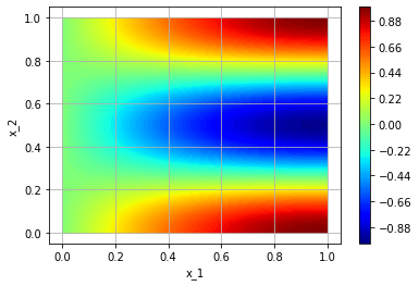
If we want to have a look on our solution, we can use the plot-methods of TorchPhysics:
plot_sampler = tp.samplers.PlotSampler(plot_domain=square, n_points=600, device='cuda')
fig = tp.utils.plot(model, lambda u : u, plot_sampler, plot_type='contour_surface')
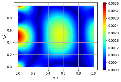
We can plot the error, since we know the exact solution:
def plot_fn(u, x):
    exact = torch.sin(np.pi/2*x[:, :1])*torch.cos(2*np.pi*x[:, 1:])
    return torch.abs(u - exact)
fig = tp.utils.plot(model, plot_fn, plot_sampler, plot_type='contour_surface')
Now you know how to solve a PDE in TorchPhysics, additional examples can be found under the example-folder.
And more in-depth information can be found on the tutorial page.